25 Homework 8: Sample Size Calculation for Two-Sample Problems

Summary

In the one-sample setting, we worked out how large a sample we need to estimate a mean to a given precision. Here we do the same for two-sample problems: how large a sample do we need to estimate a difference or ratio of group means? The tools are the same—variance formulas and the normal approximation—but the algebra gets a little more involved.

Calculus Review: Linear Approximation

We’re going to be using linear approximation to simplify some of our calculations. Given a function $f(x)$, we can approximate it near any point $x_0$ like this. \[ f(x) \approx f(x_0) + f'(x_0)(x-x_0) \]

Hopefully you remember that from calculus. If you like, you can call this first-order Taylor approximation. And there are a few formulas for the error of this approximation, which is called the remainder in Taylor’s Theorem, in most calculus textbooks.

When we’re thinking about functions of multiple variables, we use the multivariate version, which involves partial derivatives. \[ \begin{aligned} f(x,y) &\approx f(x_0,y_0) + \qty[\frac{\partial f}{\partial x}(x_0,y_0)] (x-x_0) \ + \ \qty[\frac{\partial f}{\partial y}(x_0,y_0)] (y-y_0). \end{aligned} \]

Variance Calculation for Comparisons

Differences in Means

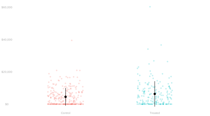
Jittered 1978 incomes for National Supported Work participants in control and treated groups, with each group mean plus or minus one standard deviation. — Figure 28.1: 1978 income for participants in the National Supported Work Demonstration.

In our Lecture on Comparing Two Groups, we talked about how to use subsample means to compare two groups. In particular, we talked about the case that we’ve drawn a sample $(X_1,Y_1) \ldots (X_n,Y_n)$ with replacement from a population $(x_1,y_1) \ldots (x_m,y_m)$ in which $x_j \in \{0,1\}$ indicates membership in one of two groups, e.g. treated and control groups in Figure 28.1. And we talked about using the difference $\textcolor[RGB]{0,191,196}{\hat\mu(1)}-\textcolor[RGB]{248,118,109}{\hat\mu(0)}$ in the mean of $Y_i$ for the subsamples in which $\textcolor[RGB]{0,191,196}{X_i=1}$ and $\textcolor[RGB]{248,118,109}{X_i=0}$ to estimate the corresponding difference $\textcolor[RGB]{0,191,196}{\mu(1)}-\textcolor[RGB]{248,118,109}{\mu(0)}$ in the population.

Throughout this section, we work conditional on the event $A=\{N_0>0,N_1>0\}$ that both subsample means exist. We suppress ``$\mid A$’’ in the expectations and variances below to keep the notation readable.

Exercise 28.1

We showed that an individual subsample mean $\hat\mu(x)$ is an unbiased estimator of the corresponding population mean $\mu(x)$. That implies that the difference of two such estimates, $\hat\mu(1)-\hat\mu(0)$, is an unbiased estimator of the difference of the corresponding population means, $\mu(1)-\mu(0)$.

Explain why the first implies the second. A sentence or even a couple words should do.

We also calculated a formula for the variance of a subsample mean $\hat\mu(x)$. \[ \mathop{\mathrm{\mathop{\mathrm{V}}}}[\hat\mu(x)] = \frac{\sigma^2(x)}{N_x} \text{ for } N_x = \sum_{i}1_{=x}(X_i) \qand \sigma^2(x) = \mathop{\mathrm{\mathop{\mathrm{V}}}}[Y_i \mid X_i=x] \]

And I stated without proof a formula for the variance of the difference of two subsample means. \[ \mathop{\mathrm{\mathop{\mathrm{V}}}}\qty[\hat{\mu}(1)-\hat{\mu}(0)] = \mathop{\mathrm{E}}\qty[\frac{1}{N_1}\sigma^2(1)+\frac{1}{N_0}\sigma^2(0)] \text{ for } N_x = \sum_{i}1_{=x}(X_i) \]

It’s a simple formula. The variance of the difference in means is the sum of the variances of the two means. Why is that the case? To start to see why, we can start from definitions and do a bit of arithmetic.

\[ \begin{aligned} \mathop{\mathrm{\mathop{\mathrm{V}}}}\qty[\hat{\mu}(1)-\hat{\mu}(0)] &= \mathop{\mathrm{E}}\qty[ \qty(\{\hat{\mu}(1) - \hat{\mu}(0)\} - \{\mu(1)-\mu(0)\})^2 ] \\ &= \mathop{\mathrm{E}}\qty[ \qty(\{\hat{\mu}(1) - \mu(1)\} - \{\hat{\mu}(0) -\mu(0)\})^2 ] \\ &= \mathop{\mathrm{E}}\qty[ \qty(\{\hat{\mu}(1) - \mu(1)\})^2 ] + \mathop{\mathrm{E}}\qty[ \qty(\{\hat{\mu}(0) -\mu(0)\})^2 ] \\ &- 2\mathop{\mathrm{E}}\qty[ \{\hat{\mu}(1) - \mu(1)\}\{\hat{\mu}(0) -\mu(0)\}] \end{aligned} \tag{28.1}\]

The first two terms here are the ones that appear in our formula above: the variances of the two means. For that formula to be correct, the last term has to be zero. It’s up to you to prove that.

Exercise 28.2

Complete the argument by proving that the ‘cross term’ is zero, i.e., that \[ \mathop{\mathrm{E}}\qty[\{\hat{\mu}(1) - \mu(1)\}\{\hat{\mu}(0) -\mu(0)\}] = 0. \]

A Tip.

Look over the calculation we used for one subsample mean $\hat{\mu}(x)$ here. You’ll want to use a lot of the same ideas: writing sums over our subsamples as sums over $1 \ldots n$ by putting in group indicators $1_{=x}(X_i)$, conditioning on $X_1 \ldots X_n$, the indicator trick, thinking about what happens when $j=i$ and $j\neq i$ in the double sum we get when we expand the product, etc. In the subsample mean calculation, the $j=i$ terms gave us some stuff that was nonzero. Why isn’t that happening here?

A Common Mistake

I saw a lot of you guys claim that $\hat\mu(0)$ and $\hat\mu(1)$ are independent in your submission. Sometimes that claim wasn’t justified; sometimes it was justified by the claim that the subsamples $\{ (X_i,Y_i) \ : \ X_i=0\}$ and $\{ (X_i, Y_i) \ : \ X_i=1 \}$ are independent. That’s not true. One way of seeing that the subsamples aren’t independent is to notice that the numbers $N_0$ and $N_1$ of observations in these subsamples sum to $n$, so if you know one you know the other. The means do, however, have zero covariance. That’s the point of this exercise, but it does take a little calculation to show it.

Ratios of Means

If $\hat\mu(1)-\hat\mu(0)$ is a good estimator of $\mu(1)-\mu(0)$, then shouldn’t $\hat\mu(1)/\hat\mu(0)$ be a good estimator of $\mu(1)/\mu(0)$? Let’s look into it. To do this, we’ll think of the ratio as a function of the two means. \[ \frac{\hat\mu(1)}{\hat\mu(0)} - \frac{\mu(1)}{\mu(0)} = f(\hat\mu(1), \hat\mu(0)) - f(\mu(1), \mu(0)) \qfor f(x,y) = \frac{x}{y}. \]

And we’ll use a linear approximation to this function to think about this difference.

\[ \begin{aligned} f(\hat\mu(1), \hat\mu(0)) \approx f(\mu(1), \mu(0)) &+ \qty[\frac{\partial f}{\partial x}(\mu(1), \mu(0))](\hat\mu(1) - \mu(1)) \\ &+ \qty[\frac{\partial f}{\partial y}(\mu(1), \mu(0))](\hat\mu(0) - \mu(0)) \end{aligned} \]

This approximation should be good if $\hat\mu(1)$ and $\hat\mu(0)$ are close to $\mu(1)$ and $\mu(0)$.

Exercise 28.3

When our sample includes a reasonably large number of observations in both groups, it’s reasonable to expect that they should be close. With a sentence or two, or a rough sketch if you prefer, explain why.

Now that we’ve justified the approximation, let’s use it to analyze our ratio estimator.

Exercise 28.4

Write out a formula for the linear approximation to the ratio estimator $\hat\mu(1)/\hat\mu(0)$ in terms of $\mu(0)$, $\mu(1)$, $\hat\mu(1)-\mu(1)$, and $\hat\mu(0)-\mu(0)$. Then approximate its bias by comparing the expected value of this linear approximation to the estimation target $\mu(1)/\mu(0)$.

Exercise 28.5

By calculating the variance of the linear approximation to $\hat\mu(1)/\hat\mu(0)$ you used in Exercise 28.4, find a formula approximating the variance of this ratio estimator. Use it to calculate a 95% confidence interval based on normal approximation for the ratio $\mu(1)/\mu(0)$ in the National Supported Work Demonstration. Draw it on top of the plot of that estimator’s bootstrap sampling distribution in Figure 2.¹ With all these approximations, are you still getting an interval similar to the one I already drew there, which is calibrated using the bootstrap?

You’ll need some information included in a table in our discussion of this study in lecture.

All of that ignores the error of our linear approximation as a potential problem. We should, if we like, be able to reason about this error using tools from calculus.

Exercise 28.6

Extra Credit. Using some version of Taylor’s Theorem to characterize the error of the linear approximation you’ve been working with, refine your answer to Exercise 28.4: find an upper bound on the absolute value of the estimator’s bias. This should be a formula involving $\mu(1)$, $\mu(0)$, and the subsample sizes $N_1$ and $N_0$. Compare it to your approximation of the estimator’s standard deviation from Exercise 28.5. Are you worried that confidence intervals like the one you calculated in Exercise 28.5 might have coverage well below the nominal level of 95%?

Sample Size Calculation for Two-Sample Problems

In the one-sample case, we used the formula $\text{se} = \sigma/\sqrt{n}$ to figure out how large a sample we needed for a given interval width. Now we want to do the same thing for the difference in means $\hat\mu(1) - \hat\mu(0)$.

The variance of the difference is $\mathop{\mathrm{E}}[\sigma^2(1)/N_1 + \sigma^2(0)/N_0]$. The subsample sizes $N_1$ and $N_0$ aren’t fixed — they depend on our sample. But on average, if a fraction $\pi$ of the population is in group 1, then $N_1 \approx n\pi$ and $N_0 \approx n(1-\pi)$. So the variance of the difference is approximately \[ \frac{\sigma^2(1)}{n\pi} + \frac{\sigma^2(0)}{n(1-\pi)} = \frac{1}{n}\qty{\frac{\sigma^2(1)}{\pi} + \frac{\sigma^2(0)}{1-\pi}}. \]

Exercise 29.1 (Part A)

Using the NSW data, estimate the quantities $\sigma^2(1)$, $\sigma^2(0)$, and $\pi$ from the sample. Then calculate approximately how large a sample you’d need to get a 95% confidence interval for $\mu(1) - \mu(0)$ with a half-width of no more than $500.

Exercise 29.2 (Part B)

Compare the sample size you calculated above to what you’d need if you were estimating a single group mean $\mu(1)$ with the same half-width. Why is the two-sample problem harder?

Exercise 29.3 (Part C)

Verify your sample size calculation by simulation. Draw 10,000 samples of size $n$ (using the $n$ you calculated in Part A) with replacement from the NSW data. For each, compute the difference in means $\hat\mu(1) - \hat\mu(0)$ and a 95% normal-approximation confidence interval. Report: (1) the average half-width, and (2) the fraction of samples where the half-width is no more than $500.

You can find the figure in the ‘Variance Calculations for Comparisons’ tab at the top of this page. Draw in your interval however you like. You can print this, draw it on paper, and photograph it for submission. You can right click on the plot, save it as an image, and draw on that using your favorite image editor. You can sketch what you see in Figure 2 on paper, add your interval, and photograph that. Maybe the easiest thing to do is use the Tldrawe Chrome Extension to draw right on top of this webpage and take a screenshot. Don’t work too hard. A rough sketch is fine.↩︎