21  Meeting 15: When Normal Breaks Down — Poisson Approximation and Quality Control

T Oct 20

$$ \newcommand{X}{} \newcommand{Y}{}

$$

The Central Limit Theorem describes what happens as the number of observations grows while the distribution of each observation stays fixed. It does not say every count based on a large sample is already close to normal.

Rare events create the important failure. If each observation is one with probability \(\theta=.01\), then a sample of \(n=100\) has an expected count of only \(n\theta=1\). The count cannot be negative, most of its probability sits on the first few integers, and its distribution is strongly skewed. A symmetric normal curve has the wrong geometry.

The brewery problem makes that failure consequential: the approximation determines whether a million-bottle delivery gets rejected.

Quality Control: The Brewery Problem

A brewer delivers a batch of a million bottles to its distributor. The distributor has recently been getting complaints, so they’ve instituted a new quality control process to try to ensure that the proportion of bad bottles is 2% or less. They set aside a hundred bottles, drawn without replacement from that million, for testing. And they find that 3 of them—3%—is bad. Having done this, they claim that the batch doesn’t meet its standards and refuse to pay. The brewer has called you in to consult.

ExercisePart A

The distributor is claiming that, on the basis of their test, they’re confident that the proportion of bad bottles in the million delivered exceeds 2%. Are you? Explain why or why not.

You’ll probably want to use the plots below. These are plots of the sampling distribution of the sample proportion \(\hat\theta=\frac{1}{100}\sum_{i=1}^{100} Y_i\) when \(Y_1 \ldots Y_{100}\) are sampled without replacement from a binary population of size 1 million in which the proportion \(\theta\) of 1s is \(.02\), \(.015\), and \(.01\).

for θ=.02

for θ=.015

for θ=.01

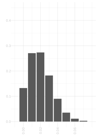
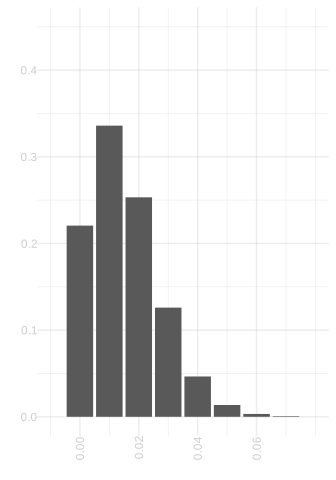
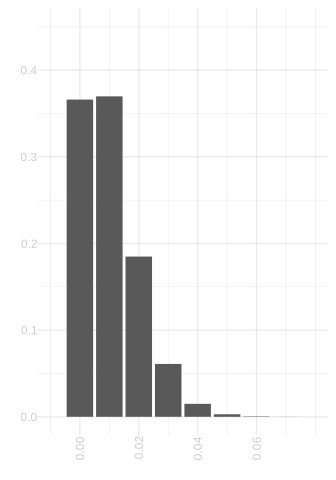
Choosing a Sample Size

ExercisePart B

The brewer claims, based on its own testing, that the proportion of bad bottles in their deliveries will be no more than 1%. You learn that the distributor will be rejecting deliveries whenever the proportion of bad ones in the sample they test exceeds 2% and, after consulting with the brewer, you decide that the best course of action is to ask them to adjust the size of their sample so they’ll reject no more than 5% of deliveries. Assuming the brewer is correct about their proportion of bad bottles, which of the following is a good sample size to ask for: 100, 400, or 1600?

The Normal Approximation Breaks Down

Write \(K=n\hat\theta\) for the number of bad bottles in the sample. If sampling from the million-bottle batch were replaced by independent sampling with replacement, then \(K\) would be Binomial with parameters \(n\) and \(\theta\).

For \(n=100\) and \(\theta=.01\), its mean is \(1\) and its standard deviation is about \(1\). That means the lower end of a two-standard-deviation normal interval is negative, even though a count cannot be. The problem is not that \(100\) sounds small. The problem is that the expected count \(n\theta\) is small.

Exact and approximate probabilities for the number of bad bottles when n=100 and θ=.01.

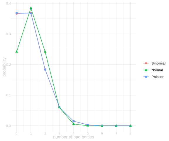
The normal approximation puts too little probability at zero and too much around the middle. If we approximate \(\Pr(K>2)\) directly by the normal tail beyond \(2\), we get about 16%, twice the Binomial probability of about 8%. A continuity correction moves the normal cutoff from \(2\) to \(2.5\) and brings the answer down to about 7%. That rescue depends on remembering that a continuous curve is standing in for discrete bars.

The Poisson approximation keeps the features the normal approximation loses. It is a distribution on nonnegative integer counts, and it can be strongly skewed. When \(n\) is large, \(\theta\) is small, and the expected count \(n\theta\) is moderate, a Binomial count is approximately Poisson with mean \(\lambda=n\theta\).

In the plot, the Poisson and Binomial points are nearly on top of each other. The Poisson estimate of the rejection probability is about 8%, matching the Binomial calculation to the displayed precision.

The Poisson Distribution

A Poisson random variable \(P\) with mean \(\lambda\) has probabilities \[ \Pr(P=k)=e^{-\lambda}\frac{\lambda^k}{k!}, \qquad k=0,1,2,\ldots. \] Its mean and variance are both \(\lambda\), so its standard deviation is \(\sqrt\lambda\). The single number \(\lambda\) therefore determines both its location and its spread.

ExerciseThe Three Candidate Sample Sizes

If the true bad-bottle proportion is \(.01\), rejection occurs when the observed proportion is greater than \(.02\). Compare the three candidate sample sizes using the Poisson approximation. Which is the smallest with rejection probability below 5%?

sample size	expected bad	first rejected count	Poisson rejection probability
100	1	3	0.080
400	4	9	0.021
1600	16	33	0.000

The choice between approximations is about the shape of the random quantity, not a slogan about sample size.

• For a rare-event count with moderate \(n\theta\), Poisson preserves discreteness and skewness.
• When both \(n\theta\) and \(n(1-\theta)\) are large, the count is far from either boundary and a normal approximation becomes more plausible.
• Sampling without replacement adds dependence. Here the population is so much larger than the sample that the Binomial and Hypergeometric distributions are practically the same, but that need not be true when the sampling fraction is large.

Takeaways

The normal approximation can fail even when the raw sample size sounds large. For rare events, the expected count \(n\theta\) is the more useful scale.

The Poisson distribution is designed for this geometry: nonnegative integer counts with mean and variance \(\lambda=n\theta\). In the brewery example it tracks the exact count probabilities much better than the normal approximation.

Next we will return to Stein’s method. The normal and Poisson distributions have different characterizing equations, but the same strategy turns each equation into a quantitative approximation bound.