11  Homework — Random Variables, Moments, and the Standard Deviation

Reminder: put each answer in its answer block. Working on paper is fine—photograph it and include it with ![](photo.png) (image in the same folder as this file).

Warm-up: Computing Moments

Exercise 12.1 (One Deck, Two Sampling Mechanisms)  

Exercise

Draw three cards from a standard deck. Do every calculation twice: first replace and reshuffle each card before the next draw; then deal three cards without replacement. Let \(I_i\) indicate that card \(i\) is a heart, and let \(H=I_1+I_2+I_3\).

  1. Calculate \(\E[H]\) in both designs. Explain why the answer is the same even though only one design has independent indicators.
  2. Calculate \(\Var(H)\) with replacement by centering and squaring out the sum.
  3. Without replacement, calculate \(\E[I_1I_2]\) and compare it with \(\E[I_1]\E[I_2]\). Use the difference to calculate \(\Cov(I_1,I_2)\).
  4. Use the three variances and six ordered cross-terms to calculate \(\Var(H)\) without replacement. Which design is more precise, and where does the difference enter?
  5. Recover \(\E[H^2]\) in both designs from your means and variances.
  6. In each design, use Markov and Chebyshev to bound the probability of drawing three hearts. Then calculate the exact probability. What information does the exact calculation use that the two moment bounds discard?

Recognition

Exercise 13.1 (What Is Independent?)  

Exercise

For each pair, say whether the two random variables are independent and identify the random mechanism that makes your answer true.

  1. The numbers shown on two separately rolled dice.
  2. Two successive cards dealt from one shuffled deck.
  3. Two separate fair coin flips.
  4. Two odds-and-evens players who each flip a separate independent fair coin.
  5. Two odds-and-evens players when the second player copies the first.
  6. The sum of two dice and the number on the first die.

Same Move, Many Surfaces

Exercise 14.1 (Variance of a Sum, the Conventional Way)  

Exercise

Let \(Y_1 \ldots Y_n\) be independent random variables with means \(\mu_1 \ldots \mu_n\) and finite variances.

  1. Center \(\sum_iY_i\), square out the centered sum, and take expectations term by term.
  2. Explain exactly where independence is used and why every off-diagonal term is zero.
  3. Conclude that \(\Var(\sum_iY_i)=\sum_i\Var(Y_i)\).
  4. Compare this proof with the independent-copy proof from class. Which step is genuinely different, and which algebra merely appears in a different place?
  5. If \(A,B,C\) are independent, use the operational rule for independence to explain why \(A+B\) and \(C\) are independent.

Indicator Counting (Cards)

The indicator-counting technique in this section follows Blitzstein and Hwang, Introduction to Probability, 2nd ed. (2019), Chapter 4.

Exercise 15.1 (Count Without Finding the Distribution)  

Exercise

Deal five cards from a shuffled standard deck without replacement.

  1. Let \(H\) be the number of hearts in the hand. Write \(H\) as a sum of five indicators.
  2. Use linearity to calculate \(\E[H]\). Why does the dependence among the five indicators not matter for this calculation?
  3. Repeat the calculation for the number of aces.
  4. Generalize both answers to a hand of \(k\) cards.
  5. Which corresponding variance calculation would require information that linearity alone does not provide?

Tell a Story

Exercise 16.1 (Tell a Story About a Joint Distribution)  

Exercise

The random pair \((A,B)\) takes values in \(\{1,2\}\times\{1,2\}\). Its joint probabilities are \[ P(A=1,B=1)=P(A=2,B=2)=\frac12, \qquad P(A=1,B=2)=P(A=2,B=1)=0. \]

  1. Tell a concrete story whose random pair has this joint distribution.
  2. Calculate the marginal distributions of \(A\) and \(B\).
  3. Someone sees only the two margins and says both variables look fair. What did they miss?
  4. Give a second joint distribution with the same margins in which \(A\) and \(B\) are independent.

Bias and Consistency

Using Prior Information

So far, we’ve exclusively talked about unbiased estimators. That is, estimators with the property that their expected value is equal to the estimation target. \[ \hat\theta \qqtext{ is called unbiased if } \E[\hat{\theta}] = \theta. \] We say an estimator is biased if this isn’t true. To get a sense of what that means, let’s consider a simple example of a biased estimator. \[ \tilde{Y}_1 = \frac{1}{n+1}\cdot \{\frac{1}{2} + \sum_{i=1}^{n}Y_i\} \]

Exercise 17.1  

Exercise

Calculate the expected value of the estimator \(\hat\theta =\tilde{Y}_1\). Then calculate its bias \(\E[\hat\theta] - \theta\) and its standard deviation \(\sqrt{\Var[\hat\theta]}\). Report all three.

This is a specific example of a more general estimator that integrates information from a prior study. Maybe a real study or maybe a study we’re imagining. Suppose we have \(\nprior\) observations \(\yprior_1 \ldots \yprior_{\nprior}\) from this study1 \[ \thetaprior = \frac{1}{\nprior}\sum_{i=1}^{\nprior}\yprior_i. \]

Then averaging all our observations — from our current study and this prior one — gives us the following estimator.

\[ \begin{aligned} \tilde{Y}_{\nprior} &= \frac{1}{\nprior + n} \qty{\sum_{i=1}^{\nprior}\yprior_i + \sum_{i=1}^{n} Y_i} \\ &= \frac{1}{\nprior + n} \qty{ \nprior\thetaprior + n\bar Y } \end{aligned} \]

We treat these prior observations, and therefore their mean \(\thetaprior\), as deterministic. The simple example we started with, \(\tilde{Y}_1\), is a special case where we have a single prior observation \(\yprior_1 = \frac{1}{2}\).

Exercise 17.2  

Exercise

Repeat Exercise 20.1 for \(\tilde{Y}_{\nprior}\).

Visualizating the Impact of Prior Information

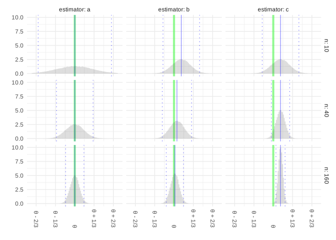
Lets’s try to get a sense of how using prior information like this impacts our inference. We’ll do it visually. The plot below shows the sampling distributions of three estimators of a population mean \(\theta\) at three sample sizes \(n\): 10, 40, and 160. These are the estimators.

  1. The estimator \(\hat\theta_1 = \tilde{Y}_{\nprior}\) for \(\thetaprior=3/4\) and \(\nprior=10\) prior observations.
  2. The estimator \(\hat\theta_2 = \tilde{Y}_{n}\) for \(\thetaprior=3/4\) and \(\nprior=n\) prior observations—the bigger the sample, the more prior observations we incorporate.
  3. The sample mean, \(\hat\theta_3 = \bar Y\).

As usual, the estimation target \(\theta\) is indicated by a green line, the sampling distribution’s mean by a solid blue line, and its mean plus and minus two standard deviations by dotted blue lines. In our first exercise, we’ll match estimators to pictures.

Exercise 17.3  

Exercise

What is the correspondence between \(\theta_1\), \(\theta_2\), and \(\theta_3\) described above and ‘estimator a’, ‘estimator b’, and ‘estimator c’ from the plot?

Nine sampling distributions arranged by sample size (10, 40, and 160) and estimator (a, b, and c). A green line marks the target, a solid blue line marks each distribution's mean, and dotted blue lines mark two standard deviations on either side.

Figure 17.1

Convergence in Probability

Now let’s think about another notion of convergence. If an estimator’s sampling distribution ends up in the right location (\(\text{bias} \to 0\)) with arbitrarily little spread (\(\text{variance} \to 0\)), then it makes sense that any draw from it will be close to the estimation target \(\mu\).

Recall that you can visualize your estimator as a single dot drawn from its sampling distribution. Like the black one below. And if you want to think of what happens if you were to repeat your survey 100 times, you can visualize the results by plotting 100 dots. Like the purple ones.
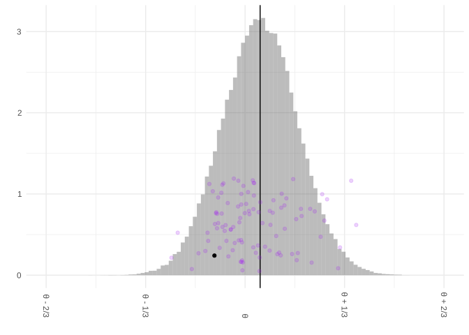
Sampling distribution for estimator b at sample size 40, with one black draw and 99 purple draws plotted over the histogram; a vertical line marks the distribution's mean.

We formalize this idea by talking about convergence in probability. We say an estimator \(\hat\mu\) converges in probability to \(\mu\) if, for anyone’s idea of `sufficiently close’, the probability that \(\hat\mu\) is sufficiently close to \(\mu\) goes to one. Or equivalently, the probability that it isn’t sufficiently close goes to zero. \[ P(\lvert\hat\mu - \mu\rvert \ge \epsilon) \to 0 \qqtext{ as } n \to \infty \]

Convergence in mean square implies convergence in probability. Let’s see why. We’ll use Markov’s inequality.

Markov’s Inequality

Markov’s inequality says that the probability a nonnegative random variable \(X\) exceeds some threshold \(t\) is bounded by the ratio of its expected value and \(t\), i.e., \[ P(X \geq t) \leq \frac{\E[X]}{t}\] Often, instead of using this to bound the random variable we’re interested in directly, e.g. \(X=\lvert\hat\mu - \mu\rvert\), we use it to bound its square. \(X \ge t\) if and only if \(X^2 \ge t^2\), so the probability that \(X \ge t\) is the same as the probability that \(X^2 \ge t^2\). Applying Markov’s inequality to the random variable \(X^2\) gives us a bound in terms of \(X\)’s mean square. \[ P(X \ge t) = P(X^2 \ge t^2) \leq \frac{\E[X^2]}{t^2} \qqtext{ e.g.} P(\lvert\hat\mu - \mu\rvert \ge \epsilon) = P((\hat\mu - \mu)^2 \ge \epsilon^2) \leq \frac{\E[(\hat\mu - \mu)^2]}{\epsilon^2} \]

This tells us, in terms of the mean squared error of \(\hat\mu\), how likely it is that \(\hat\mu\) is far from \(\mu\). And, in particular, it tells us that if the mean squared error goes to zero, then the probability that \(\hat\mu\) is any distance \(\epsilon\) away from \(\mu\) goes to zero.

Now we’re going to do two things. First, we’re going to prove Markov’s inequality. It’s good practice working with expectations and probabilities. Second, we’re going to look at what Markov’s inequality tells us about how close \(\hat\mu\) is to \(\mu\), i.e., we’re going to use it to calculate the coverage of an interval estimate.

First we define the following two functions, \(f\) and \(g\), with \(t, x\ge 0\). \[ f(x,t) = \frac{x}{t} \] \[ g(x,t) = 1_{\ge t}(x) = \begin{cases} 1 & \text{ if } x \ge t \\ 0 & \text{ otherwise } \end{cases} \]

Exercise 18.1  

Exercise

We pick \(t=3\), plot the two functions above on the same coordinate with \(x\) on the x axis. Based on the graph, what can we infer about the relationship between \(f(x,t)\) and \(g(x,t)\)?

Exercise 18.2  

Exercise

It turns out that your inference is correct! For all \(t, x\ge 0\), \(\frac{x}{t} \ge 1_{\ge t}(x)\). Use the fact to prove Markov’s inequality.

Hint 1. \(\E[Y]\ge \E[Z]\) if \(Y\ge Z\)

Hint 2. Knowing that \(\frac{x}{t} \ge 1_{\ge t}(x)\), we can infer that \(\frac{X}{t} \ge 1_{\ge t}(X)\) for \(X\) being a non-negative random variable.

Markov’s Inequality and Interval Estimation

So far, when we’ve calculated the coverage of an interval estimate in terms of its mean and variance, we’ve relied on normal approximation. That is, we’ve been using a different formula for \(P(\lvert\hat\mu - \mu\rvert \ge \epsilon)\) based on the idea that \(\hat\mu-\mu\) has approximately the same distribution as a normally-distributed random variable \(Z\) with the same mean—zero—and variance \(\sigma_{\hat\mu}^2=\Var[\hat\mu-\mu]\). We can use this approximation, in combination with our knowledge of the probability density of the normal approximation, to get a bound on the probability that \(\lvert\hat\mu - \mu\rvert \ge \epsilon\).

\[ P(\abs{\hat\mu - \mu} \ge \epsilon) \approx P(\abs{Z} \ge \epsilon) = 1-P(\abs{Z} < \epsilon) = 1- \int_{-\epsilon}^{\epsilon} f_{\sigma_{\hat\mu}}(z) dz \qfor f_{\sigma}(z) = \frac{1}{\sqrt{2\pi}\sigma} e^{-z^2/(2\sigma^2)} \]

The reason we’re always talking about intervals of the form \(\hat\mu \pm 2 \sigma_{\hat\mu}\) is that, using this approximation, that yields 95% coverage. That is, \(P(\abs{Z} < 2 \sigma_{\hat\mu}) \approx .95\). To see why we tend to use normal approximation instead of Markov’s inequality, let’s see what Markov’s inequality tells us about how close an estimator is to its estimation target and about the coverage of this interval.

Exercise 18.3  

Exercise

To see what Markov’s inequality can tell us, first we can apply the property to the squared deviation from the mean: \[ X = \{\hat{\theta}-\E[\hat{\theta}]\}^2 \] \[ P(X\ge t)\le \frac{\E[\{\hat{\theta}-\E[\hat{\theta}]\}^2]}{t} = \frac{\Var(\hat{\theta})}{t} \]

When we do this, what does Markov’s inequality tell us about how close our estimator is to its mean? What is the probability that it’s within 1, 2, 3 standard deviations?

Exercise 18.4  

Exercise

We can use this to calibrate an interval. What does it tell us about the probability that \(\hat{\theta} \pm 2 \sigma_{\hat{\theta}}\) contains \(\E[\hat{\theta}]\)? How wide must an interval of width \(w\) be so that \(\hat{\theta} \pm \frac{w}{2}\) has 95% coverage?

Hint. \(\hat{\theta} \pm \frac{w}{2}\) contains \(\theta\) if and only if \(|\hat{\theta}-\theta| \le \frac{w}{2}\). Therefore, \(P(\hat{\theta} \pm \frac{w}{2} \text{ contains } \theta) = P(|\hat{\theta}-\theta| \le \frac{w}{2})\).

Comparing Interval Calibration Methods

Exercise 19.1 (Exact and Guaranteed Intervals)  

Exercise

Return to the binary population and sample size from the earlier calibration homework. Use the exact Binomial method from that homework and the Chebyshev method from this week’s chapter.

  1. Derive the value \(t\) for which Chebyshev guarantees \(P(|\hat\theta-\theta|\le t\sigma)\ge .95\).
  2. On the same axis, draw the exact middle-95% interval for \(\hat\theta\) and the guaranteed interval \(\theta\pm t\sigma\).
  3. Compare their widths over a grid of values of \(\theta\). Which method needs the full distribution, and which needs only the first two moments?
  4. Explain why the guaranteed interval is useful even though it is much wider.
  5. Save this comparison. After normal approximation, add the normal interval to the same object rather than starting a new exercise.

Exercise 19.2 (Coverage Is an Empirical Question)  

Exercise

Let \(\theta=.7\) and draw binary samples of size \(n=625\). For each sample, calculate both the sample mean \(\bar Y\) and the pseudo-observation estimator \(\tilde Y_{\nprior}\) from Exercise 20.2 with \(\nprior=100\) and \(\thetaprior=.5\).

  1. For each estimator, construct three intervals centered at the observed point estimate: a 95% bootstrap interval, a 95% normal-approximation interval, and an interval whose radius is \(\sqrt{20}\) times the estimated standard deviation. For the pseudo-observation estimator, estimate its standard deviation by replacing \(\theta\) with \(\bar Y\) in the variance formula you derived earlier. The last radius is Chebyshev-calibrated around the estimator’s expectation; for the biased estimator, it does not guarantee 95% coverage of \(\theta\).
  2. Repeat the experiment 1,000 times. For each of the six estimator-and-calibration pairs, report empirical coverage and average width.
  3. Which calibration method would you use for each point estimator? Separate the question “is the interval narrow?” from “does it cover \(\theta\) 95% of the time?”
  4. Repeat with \(n=2500\). Explain why increasing the amount of real data changes both the bias and the variance advantage of the pseudo-observations.

Exercise 19.3 (One More Moment)  

Exercise

Let \(X\) equal one with probability \(p\) and zero with probability \(1-p\).

  1. List the two possible values of \(|X-p|^3\) and their probabilities.
  2. Calculate \(\E|X-p|^3\).
  3. For \(n\) independent copies, calculate the sum of the \(n\) individual third absolute centered moments.
  4. The later normal-approximation result uses this sum. Why is that easier than calculating the distribution—or the third absolute centered moment—of the sum itself?

Paley–Zygmund: The Other Half

Exercise 20.1 (Bonus: A Lower Bound on Spread)  

Exercise

For a nonnegative random variable \(Z\) and \(0<a<1\), the Paley–Zygmund inequality says \[ P(Z\ge a\E Z)\ge (1-a)^2\frac{(\E Z)^2}{\E[Z^2]}. \] Let \(Y\) have mean \(\mu\), positive variance \(\sigma^2\), and finite fourth centered moment. Apply the inequality with \(Z=(Y-\mu)^2\) and \(a=1/2\).

  1. Rewrite the event \(Z\ge a\E Z\) as a statement about \(|Y-\mu|\) and \(\sigma\).
  2. Express the resulting lower bound using \(\sigma^4\) and \(\E[(Y-\mu)^4]\).
  3. Chebyshev says there cannot be too much probability far from \(\mu\). Explain how this result says that the standard deviation cannot be describing spread that is not really there.

  1. Sometimes we call these pseudo-observations. This particular interpretation, in which we think of them as coming from a prior study, can be used to derive this estimator from Bayesian principles.↩︎