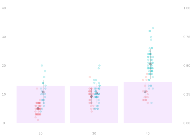
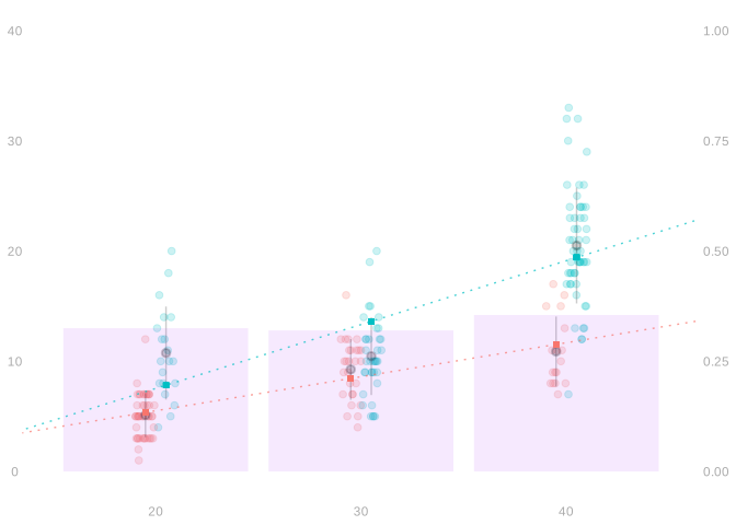
We use the same data and model from the previous meeting.
In the previous meeting, we studied the behavior of least squares predictors. We worked one direction at a time: perturb \(\hat\mu\) in a direction \(m \in \mathcal{M}\), check that the derivative of the sum of squared errors is zero. Here we express the same ideas in matrix notation. The formulas become more compact, and—more importantly—eigendecomposition lets us see all directions at once and identify which ones matter.
A sample drawn with replacement from a population.
The least squares predictor in the not-necessarily-parallel lines model.
Matrix Notation for Least Squares
Feature Vectors and Linear Models
We can write things compactly if we have notation for a vector of basis functions. \[ m_\beta(x) = \beta_0 + \beta_1 x + \beta_2 x^2 + \beta_3 x^3 = \phi(x)^T \beta \quad \text{ where } \quad \phi(x) = \begin{pmatrix} 1 \\ x \\ x^2 \\ x^3 \end{pmatrix}. \]
For example, we can write our characterization of \(\hat \mu\) on one line. \[
\hat \mu(x) = \phi(x)^T \hat\beta \quad \text{ where } \quad \hat \beta = \arg\min_{\beta \in \mathbb{R}^4} \frac{1}{n}\sum_{i=1}^n \left\{ \phi(X_i)^T \beta - Y_i \right\}^2.
\]
We often call \(\phi(x)\) the feature vector for \(x\) and its elements \(\{\phi(x)\}_j = \phi_j(x)\)features. \(A\) is for apple; think \(\phi\), the greek \(f\), for feature.
Our Example
In the previous meeting, we used the ‘not necessarily parallel lines’ model to predict \(Y\) from treatment \(W\) and covariate \(X\). The feature vector for this model is \[
\phi(w,x) = \begin{pmatrix} 1 \\ w \\ x \\ wx \end{pmatrix} \qquad \text{so} \qquad m_\beta(w,x) = \beta_0 + \beta_1 w + \beta_2 x + \beta_3 wx.
\]
Stacking the feature vectors for all \(n\) observations gives us a matrix \(\Phi\) with \(n\) rows and \(4\) columns.
None of this is specific to the cubic polynomial or not-necessarily-parallel lines model. Every linear model can be described in essentially the same way. \[
\mathcal{M} = \left\{ m(x) = \phi(x)^T \beta : \beta \in \mathbb{R}^{k+1} \right\} \text{ for some feature vector } \phi(x) = \begin{pmatrix} \phi_0(x) \\ \phi_1(x) \\ \vdots \\ \phi_{k}(x) \end{pmatrix}.
\]
We call the number of features we need, which is \(k+1\) above, the dimension of the linear model.
Since we’re always considering all coefficients \(\beta \in \mathbb{R}^{k+1}\), we can specify a model by just saying what the features are — or equivalently by giving the formula \(m_\beta(x)\).
The \(j\)th partial is the \(j\)th basis function. \[ \frac{\partial}{\partial \beta_j} m_{\beta}(x) = \phi_j(x). \]
Solving the Linear Least Squares Problem
To find the coefficients \(\hat\beta\) that minimize squared error, we set the derivatives to zero and solve. \[
\hat \beta = \arg\min_{\beta \in \mathbb{R}^{k+1}} \frac{1}{n}\sum_{i=1}^n \{ m_{\beta}(X_i) - Y_i \}^2
\] satisfies \[
\begin{aligned}
0
&= \frac{\partial}{\partial \beta_j}\vert_{\beta=\hat\beta} \ \frac{1}{n}\sum_{i=1}^n \{ m_{\beta}(X_i) - Y_i \}^2 \\
&= \frac{2}{n} \sum_{i=1}^n \phi_j(X_i) \{ \phi(X_i)^T \hat \beta - Y_i \} \quad \text{ for } \quad j=0 \ldots k.
\end{aligned}
\] Stacking these equations and rearranging, we get a linear system. \[
\underbrace{\frac{1}{n}\sum_{i=1}^n \phi(X_i) \phi(X_i)^T}_{\hat\Sigma} \hat \beta = \underbrace{\frac{1}{n}\sum_{i=1}^n \phi(X_i) Y_i}_{\phi^Y}.
\]
If \(\hat\Sigma\) is invertible, this has a unique solution. \[ \hat\beta = \hat\Sigma^{-1}\phi^Y \text{ is the unique solution}. \]
If it isn’t, the set of solutions is the analogous inverse image. \[ \text{ Every } \hat \beta \in \hat\Sigma^{-1} \{ \phi^Y \} \text{ is a solution. } \]
In the previous meeting, we studied stability by working one direction at a time. The matrix formulation lets us see all directions at once. The tool is eigendecomposition.
\[ \hat \Sigma = \sum_{k=1}^d \sigma_k u_k u_k^T \quad \text{ where } \quad \|u_k\|=1 \text{ and } \quad u_j^T u_k = 0 \quad \text{ for } j \neq k. \]
The eigenvalue \(\sigma_k\) measures how much the data varies in the direction \(u_k\). In one formula: \(\sigma_k = u_k^T \hat\Sigma u_k = \frac{1}{n}\sum_{i=1}^n \{u_k^T \phi(X_i)\}^2\).
The largest eigenvalue is much larger than the smallest. That means some directions in coefficient space are much better determined than others.
And we can represent \(\phi^Y\) and \(\hat\beta\) as linear combinations of the eigenvectors. \[ \phi^Y = \sum_{k=1}^d (u_k^T \phi^Y) u_k. \] Then one solution is \[ \hat\beta^{\text{span}} = \sum_{k : \sigma_k > 0} \sigma_k^{-1} (u_k^T \phi^Y) u_k. \]
When Coefficients are Unstable
Typically, \(\hat \Sigma\) will be invertible. Exceptions happen when
Our model is too big, i.e. has dimension \(>\) number of observations.
Our observations are precisely structured, so there is collinearity among the feature vectors \(\phi(X_1) \ldots \phi(X_n)\).
However, it may not be that invertible. If it has small eigenvalues \(\sigma_k \approx 0\), variation in the direction \(u_k\) blows up. This means our estimate of \(\hat\beta\) is very unstable. If we change \(\phi^Y\) just a little in that direction, we see big changes to the coefficient vector\(\hat \beta\). \[ \hat\beta_{\delta} = \hat\Sigma^{-1} \left(\phi^Y + \delta u_k\right) = \hat\beta + \delta \sigma_k^{-1} u_k. \]
This isn’t necessarily meaningful. We don’t really care about the coefficients \(\hat\beta\). We care about the corresponding curve \(\hat\mu(x)=\phi(x)^T \hat\beta\). That’s what we use to make predictions.
Stability of Predictions
Consider the predictions we get after a small change to \(\phi^Y\). \[
\begin{aligned}
\hat\beta_{\delta} &= \hat\Sigma^{-1} \left(\phi^Y + \delta u_k\right) = \hat\beta + \delta \sigma_k^{-1} u_k. \\
\hat\mu_{\delta}(w,x) &= \phi(w,x)^T \left(\hat\beta + \delta \sigma_k^{-1} u_k\right) = \hat\mu(w,x) + \delta \sigma_k^{-1} \phi(w,x)^T u_k.
\end{aligned}
\] This change makes a big difference in predictions at \((w,x)\) only if \(\phi(w,x)\) aligns well with a direction \(u_k\) we don’t see much of in the data, i.e. one with \(\sigma_k \approx 0\).
Let’s see what this looks like for our data. Each eigenvector \(u_k\) defines a curve \(\phi(w,x)^T u_k\). Here are its values at the six \((w,x)\) combinations in our data.
The prediction perturbation in direction \(u_k\) is \(\delta \sigma_k^{-1} \phi(w,x)^T u_k\). Directions with small eigenvalues amplify the perturbation—but only at points where \(\phi(w,x)\) aligns with that direction.
Summary: if you don’t see something much, don’t trust predictions about it.
Variance of Predictions
Signal + Noise Decomposition
Let’s return to our \(\text{signal} + \text{noise}\) model. \[ Y_i = \mu(X_i) + \varepsilon_i \quad \text{ so } \quad \phi^Y =
\underset{\phi^\mu}{\frac{1}{n}\sum_{i=1}^n \phi(X_i) \mu(X_i)}
+
\underset{\phi^\varepsilon}{\frac{1}{n}\sum_{i=1}^n \phi(X_i) \varepsilon_i}. \] We’ll think about how sensitive our prediction is to noise. \[ \hat \mu(w,x) = \phi(w,x)^T \hat \beta = \phi(w,x)^T \hat\Sigma^{-1} \phi^{\mu} + \phi(w,x)^T \hat\Sigma^{-1} \frac{1}{n}\sum_{i=1}^n \phi(X_i)\varepsilon_i. \]
Variance Derivation
The variance is \[
\begin{aligned}
\text{Var} \{\hat\mu(w,x)\}
&= E \left\{ \phi(w,x)^T \hat\Sigma^{-1} \frac{1}{n}\sum_{i=1}^n \phi(X_i)\varepsilon_i \right\}^2 \\
&= \frac{1}{n^2} \sum_{i=1}^n \{ \phi(w,x)^T \hat\Sigma^{-1} \phi(X_i)\}^2 E \varepsilon_i^2 \\
&= \frac{1}{n}\phi(w,x)^T \hat\Sigma^{-1} \hat\Sigma_{w} \hat\Sigma^{-1} \phi(w,x) \quad \text{ for } \quad \hat \Sigma_w = \frac{1}{n}\sum_{i=1}^n E \varepsilon_i^2 \phi(X_i)\phi(X_i)^T.
\end{aligned}
\]
This is a sandwich: \(\hat\Sigma^{-1} \hat\Sigma_w \hat\Sigma^{-1}\). The bread is the inverse of the feature covariance. The filling is the noise-weighted feature covariance. If \(E\varepsilon_i^2\) doesn’t depend on \(i\), the filling and the bread are proportional and the sandwich simplifies. \[ \text{Var} \{\hat \mu(w,x)\} \approx \frac{\sigma^2}{n} \phi(w,x)^T \hat\Sigma^{-1} \phi(w,x). \] This means that the better aligned \(\phi(w,x)\) is with the less visible principal components \(u_k\) (those with \(\sigma_k \approx 0\)), the bigger the variance of our prediction. In short, we can’t be precise when we haven’t seen much evidence.
Checking the Formula Against Simulation
We already simulated the sampling distribution of \(\hat\theta\) in the previous meeting. Let’s check the formula against those simulations for individual predictions \(\hat\mu(w,x)\).
The formula gives us a way to compute standard errors from a single sample. That’s what makes the matrix formulation useful in practice: confidence intervals without simulation.
Exercises: Stability in a Concrete Example
Let’s put these formulas to work in a concrete setting where we can calculate everything by hand and compare to what the theory predicts.
Setup: A Basketball Example
Suppose we’re using height to predict rebounds. We’ll work with heights rounded to the nearest inch, and at each even height \(X_i\) from 60 inches to 86 inches (5’ - 7’2”), we’ll include one player in our dataset. However, at each height there are two players we could include, one having \(2\) more rebounds than the other. If \(\mu(X_i)\) is the average number of rebounds for the two players with height \(X_i\), then we have one observation \((X_i,Y_i)\) for each \(X_i \in 60, 62, 64, \ldots 84\) and \[ Y_i = \mu(X_i) + \varepsilon_i \quad \text{ for } \quad \varepsilon_i = \pm 1. \] And we’ll flip a coin to choose between the two players at each height, so \[ Y_i = \mu(X_i) + \varepsilon_i \text{ where } \varepsilon_1 \ldots \varepsilon_n \text{ are independent with } \varepsilon_i = \begin{cases} +1 & \text{with probability $1/2$} \\ -1 & \text{with probability $1/2$} \end{cases}. \] We’re going to do least squares regression using a cubic polynomial model to predict the number of rebounds we’d see from players at other heights, like the odd heights \(61\), \(73\), and \(89\).
Exercise: Derive the Variance Formula
Calculate the standard deviation of \(\hat\mu(x)\) for arbitrary \(x\). To do this, take the following steps.
Write out a formula for \(Z=\hat \mu(x)\).
Calculate its expectation \(E Z\) and write out \(Z - E Z\).
Write out the square \((Z-E Z)^2\). This should be a double sum, as the square of a sum \(\sum_{i=1}^n z_i\) is \(\sum_{i=1}^n \sum_{j=1}^n z_i z_j\).
Now you should be ready to calculate the expected square \(\text{Var}(Z) = E(Z - E Z)^2\). The expectation of a sum is the sum of the expectation of its terms, so all you’ve got to do is compute the expectation of its terms. Are any zero? If so, why?
Try to find a nice way to express \(\text{Var}(Z)\) in terms of the feature vector \(\phi(x)\) and the covariance matrix \(\hat\Sigma = \frac{1}{n}\sum_{i=1}^n \phi(X_i)\phi(X_i)^T\).
Exercise: Check the Formula by Simulation
Let \(\mu(X_i) = X_i/4\). We can generate observations using the following R code.
Fit a cubic polynomial to this data and record the prediction \(\hat\mu(x)\) for \(x=61\). Do this 1000 times, so we have \(1000\) predictions \(\hat \mu_{1}(x) \ldots \hat \mu_{1000}(x)\) based on different random vectors \(\varepsilon=[\varepsilon_1 \ldots \varepsilon_n]\) with the same distribution. Compute the sample variance, \[ \widehat{\text{Var}}\{ \hat \mu(x) \} = \frac{1}{1000}\sum_{j=1}^{1000}\left\{\hat \mu_{j}(x) - \frac{1}{1000}\sum_{j=1}^{1000} \hat \mu_j(x) \right\}^2. \] Then compare to the variance \(\text{Var}\{ \hat \mu(x) \}\) you get using your formula from the previous exercise. If they’re not similar, there’s either a bug in your code or an error in your derivation. Work out which and fix it.
Then, once you’re done, plot a histogram of your estimates \(\hat \mu_1 \ldots \hat \mu_{1000}\). Roughly how many of these thousand observations fall within one standard deviation of the mean? What about two standard deviations?
Exercise: Other Prediction Points
Repeat the previous exercise for new heights \(x=73\) and \(x=81\). What changes? What stays the same?
Exercise: Other Models
Repeat the simulation exercises using two new models. You’ll need to generalize your variance formula to give you \(\text{sd}\{ \hat\mu(x) \}\) for any linear model \(\mathcal{M}\), i.e. for any feature vector \(\phi(x)\).
Piecewise-constant curves with breaks at \(66\), \(70\), \(74\), \(78\), and \(82\).
Cubic splines with knots at \(66\), \(70\), \(74\), \(78\), and \(82\). The R formula for a cubic spline with knots at the points \(\text{knot}_1, \text{knot}_2, \ldots \text{knot}_k\) collected into a vector knot\(\in \mathbb{R}^k\) is Y ~ bs(X, knots=knot).
Describe the differences you see when you use these different models. And try to explain where these differences come from.