28 Sampling and Randomization
$$ \newcommand{X}{} \newcommand{Y}{}
$$
Two Questions, Two Random Mechanisms
The social-pressure experiment began with a finite population of households. In the previous chapter we treated those households as fixed and studied repeated treatment assignment. That isolates randomization variability.
Often we also want an answer about a population larger than the units in one study. Then two mechanisms matter:
- Sampling determines which population units enter the study.
- Randomization determines which treatment each sampled unit receives.
The mechanisms answer different questions. Sampling connects a study sample to a population. Randomization connects observed treatment groups to causal effects.
The Process
Start with a finite population \[ \{x_j,y_j(0),y_j(1)\}_{j=1}^m. \]
First draw indices \(J_1\ldots J_n\) uniformly with replacement from \(1\ldots m\). The sampled potential outcomes are \[ Y_i(0)=y_{J_i}(0),\qquad Y_i(1)=y_{J_i}(1). \]
Then assign exactly \(n_1\) sampled positions to treatment and \(n_0=n-n_1\) to control. The realized outcome is \[ Y_i=Y_i(W_i). \]
The difference in observed means is \[ \hat\tau =\frac1{n_1}\sum_{i:W_i=1}Y_i -\frac1{n_0}\sum_{i:W_i=0}Y_i. \]
Why the Two Stages Work
Fix the sample first. Across repeated random assignments, \[ \mathop{\mathrm{E}}[\hat\tau\mid J_1\ldots J_n] =\frac1n\sum_{i=1}^n\{Y_i(1)-Y_i(0)\}. \] Randomization therefore targets the average effect in the realized sample.
Now average over repeated samples. Each sampled position is a uniform draw from the population, so \[ \mathop{\mathrm{E}}\qty[\frac1n\sum_{i=1}^n\{Y_i(1)-Y_i(0)\}] =\frac1m\sum_{j=1}^m\{y_j(1)-y_j(0)\} =\bar\tau. \]
The law of iterated expectations joins the steps: \[ \mathop{\mathrm{E}}[\hat\tau] =\mathop{\mathrm{E}}\qty[\mathop{\mathrm{E}}[\hat\tau\mid J_1\ldots J_n]] =\bar\tau. \]
Neither mechanism substitutes for the other. Randomizing a badly selected sample can identify its sample effect without making that sample representative.
Seeing the Two Sources
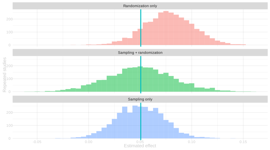
The green line is the average effect in the simulated finite population. The panels use the same horizontal scale.
- Sampling only varies who enters and calculates the sample’s complete average effect, as if both potential outcomes were visible.
- Randomization only holds one sample fixed and varies which outcome is revealed for each sampled unit.
- Sampling + randomization repeats both stages, which is the actual two-source process.
Takeaways
- Sampling variability is about who enters the study.
- Randomization variability is about which potential outcome is revealed.
- Conditioning on the sample isolates the randomization argument.
- Iterated expectation joins the sample result to the population result.
- Real GGL covariates can organize the example, but completed potential-outcome pairs must remain explicitly simulated.