9 Random Variables and Moments
============================================================================ –>
Earlier, we found the distribution of a sum by listing all the ways the sum could happen and adding their probabilities. That calculation was exact. It also sucked. Even when the two things being added had simple distributions, the sum made us build a new distribution from all their possible pairs.
Today we will add the same random quantities without doing that. A random variable gives us a handle on a distribution: we can write \(X+Y\) before we know the distribution of \(X+Y\). We can then calculate summaries such as its expectation and variance directly. Adding distributions is expensive; adding the summaries we need is often cheap.
This does not make the distribution disappear. It lets us postpone opening it. The question for this chapter is how much we can learn about a random quantity while leaving its full distribution closed.
Random Variables
A lot of this is review.
Observations as Random Variables
The notation \(y_j\) refers to a number. It’s the income of the \(j\)th person in our population. That’s just some person. The notation \(Y_i\) refers to something else. It’s the income of the \(i\)th person we call in our survey. That’s not a person. That’s the result of a random process—the roll of a die. To summarize this result, we talk about the probability distribution of \(Y_i\).
Probability Distributions
When our outcomes are binary, it’s easy to describe this distribution. All we need to know is the probability that \(Y_i\) is 1. To do that, we sum the probabilities of the rolls that result in it being one, \[ P(Y_i = 1) = \sum_{j: y_j = 1} P(\text{roll}_i = j) = \sum_{j: y_j = 1} \frac{1}{m} \times y_j = \mu. \] This collapses out information about our random process that’s irrelevant to \(Y_i\). That is, it collapses the probability we roll each number in 1…m into our ‘weighted coin flip’.
When our outcomes are nonbinary, it’s a bit more complicated. We need to know the probability that \(Y_i\) takes on each possible value. But we calculate it the same way—we sum the probabilities of the rolls that result in it taking on those values, \[ P(Y_i = y) = \sum_{j: y_j = y} P(\text{roll}_i = j). \] We’re still collapsing out irrelevant information, but what we’re left with is more complicated. It’s a weighted die roll, with one face for each possible value of \(Y_i\). And if each person’s income is different, then there’s nothing to collapse out, \[ P(Y_i = y) = \begin{cases} \frac{1}{m} & \qqtext{for} y \in y_1 \ldots y_m \\ 0 & \qqtext{otherwise} \end{cases} \]
Cumulative Distribution Functions
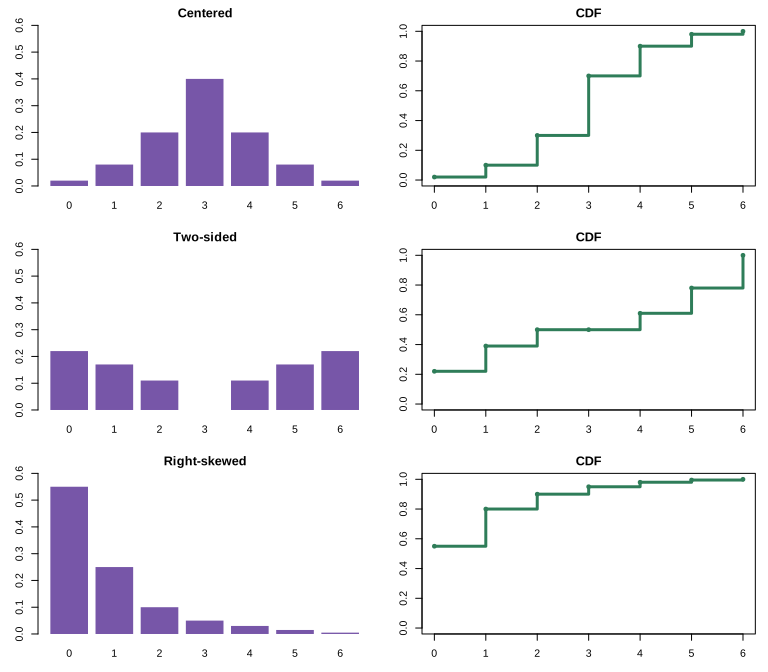
One way to package the whole distribution is its cumulative distribution function, \[ F(y)=P(Y\le y). \] This function answers every threshold question at once, and later it will let us compare a sampling distribution with a normal approximation. It is theoretically useful. It is also a terrible way to look at a random variable: every CDF starts near zero, climbs monotonically, and ends near one. Very different distributions become variations on the same rising shape. Histograms and probability-mass plots let us see the distribution’s shape; a CDF is a tool we reach for when its particular cumulative information is what we need.
Expectations
That said, we often don’t need to know the whole distribution. Often the only thing we care about is the expected value of \(Y_i\). Or some related quantity. The expected value of \(Y_i\) is the probability-weighted average of the values it can take on. What’s nice about this is that we can think of this in ‘uncollapsed’ terms. When we sample as usual, this is just the population mean. The collapsed form is, in a sense, just summing in a different order, \[ \begin{aligned} \E[Y_i] = \sum_y P(Y_i = y) \times y = \sum_y \qty(\sum_{j: y_j = y} \frac{1}{m}) \times y = \frac{1}{m}\sum_y\sum_{j:y_j = y} y = \frac{1}{m}\sum_{j=1}^m y_j. \end{aligned} \]
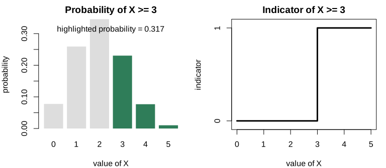
What’s nice about the binary case is, in fact, that it’s an expectation. When \(Y_i\) is binary, the probability it’s 1 is its expected value \(Y_i\), \[ \begin{aligned} P(Y_i=1) = \sum_{j: y_j = 1} P(\text{roll}_i = j) &= \sum_{j:y_j=1} \frac{1}{m} \\ &= \sum_{j=1}^m \frac{1}{m} \times \begin{cases} 1 & \ \ \text{ if } y_j = 1 \\ 0 & \ \ \text{ otherwise} \\ \end{cases} \\ &= \sum_{j=1}^m \frac{1}{m} \times y_j = \E[Y_i]. \end{aligned} \] In fact, we like expectations so much that we often use them to work with probabilities, \[ P(Z \in A) = \E[1_A(Z)] \qfor 1_A(z) = \begin{cases} 1 & \qqtext{ for } z \in A \\ 0 & \qqtext{ otherwise} \end{cases} \]
This is a principle, not a notational trick: probabilities are expectations of indicators. The indicator keeps exactly the part of the random outcome that matters for the event and throws everything else away. Its probability-weighted average is the probability that it is one. Consequently, every rule we prove for expectations is also a tool for probabilities.
Uniform-at-random sampling turns population summaries into expectations. If \(Y\) is one uniform draw from the fixed values \(y_1 \ldots y_m\), then \[ \E[Y]=\frac1m\sum_{j=1}^m y_j=\mu \qquad\text{and}\qquad \E[(Y-\mu)^2]=\frac1m\sum_{j=1}^m(y_j-\mu)^2=\sigma^2. \] The population mean and variance are therefore not new objects after we introduce random variables. The mean is the first raw moment of a uniform draw from the population, and the variance is its second central moment.
Independence
Random variables are independent if, in intuitive terms, knowing the value of one doesn’t tell us anything about the value of the other. In mathematical terms, their joint probability distribution is the product of their individual marginal ones, \[ P(Y_1 ... Y_k = y_1 \ldots y_k) = P(Y_1=y_1) \times \ldots \times P(Y_k=y_k). \] That’s what happens when the randomness in each \(Y_i\) comes from a different roll of the die. And since that’s how we’re doing our sampling in the Current Population Survey, it’ll be true in our sample. Because we draw each of our observations the same way, they also have the same probability distribution. We say they’re independent and identically distributed. At least, that’s what we’re pretending when we analyze CPS data in this class. Reality is more complicated.
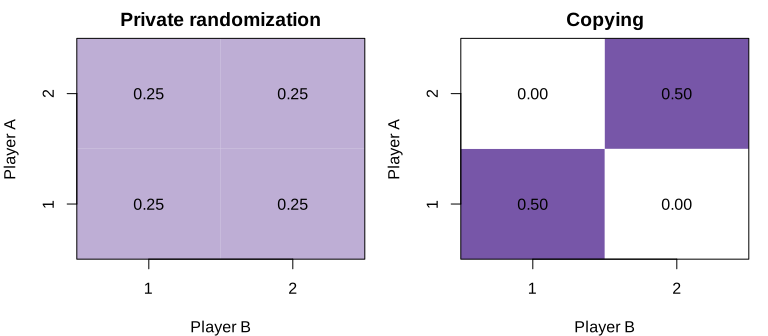
Independence lives in the joint distribution, not in either variable by itself. Suppose two players in odds-and-evens each show either one or two fingers. Under fair play, both privately randomize, so the four possible pairs have probability \(1/4\). Now suppose the player who wins on an even sum secretly copies the other player’s choice. Only \((1,1)\) and \((2,2)\) occur, each with probability \(1/2\). Each player’s individual distribution still looks perfectly fair: each shows one or two half the time. The cheating appears only in the random pair \((A,B)\). Knowing \(A\) now determines \(B\).
Sampling without replacement is the same kind of warning in a familiar setting. Each draw has the right marginal distribution, but the first draw changes what can happen on the second.
The definition is a statement about the joint distribution. The version we use in calculations is a statement about functions: if \(Y\) and \(Z\) are independent, then \[ \E[f(Y)g(Z)]=\E[f(Y)]\E[g(Z)]. \] For example, \(Y-\E Y\) and \(Z-\E Z\) are still functions of separate independent random variables. Their product therefore has expectation zero. This is the fact that will make the cross-terms disappear when we calculate the variance of a sum.
Working with Expectations
Monotonicity of Expectations
If \(a(x)\le b(x)\) for every possible value \(x\) of \(X\), then \[ \E[a(X)]\le \E[b(X)]. \] The proof is just the definition of expectation. Every difference \(b(x)-a(x)\) is nonnegative, and every probability is nonnegative, so \[ \E[b(X)]-\E[a(X)] =\sum_x \{b(x)-a(x)\}P(X=x)\ge 0. \] Next time we will use this result in a picture: draw a simple function above an indicator, then take expectations of both sides to turn the picture into a probability bound.
Linearity of Expectations
\[ \begin{aligned} E ( a Y + b Z ) &= E (aY) + E (bZ) \\ &= aE(Y) + bE(Z) \\ & \text{ for random variables $Y, Z$ and numbers $a,b$ } \end{aligned} \]
There are two things going on here. To average a sum of two things, we can take two averages and sum. To average a constant times a random variable, we multiply the random variable’s average by the constant. In other words, we can distribute expectations and can pull constants out of them.
Unbiasedness of the Sample Mean
The Sample Mean
Claim. The sample mean is an unbiased estimator of the population mean. \[ \E[\hat\mu] = \mu \]
\[ \begin{aligned} \E\qty[\frac1n\sum_{i=1}^n Y_i] &= \frac1n\sum_{i=1}^n \E[Y_i] && \text{ via linearity } \\ &= \frac1n\sum_{i=1}^n \mu && \text{ via equal-probability sampling } \\ &= \frac1n \times n \times \mu = \mu. \end{aligned} \]
The sample mean is an unbiased estimator of the population mean. Now that we’ve worked out that the location is good, it’s time to talk about spread. That’s what we’ll do next time.
Variance and Standard Deviation
Variance has two equivalent forms that reveal different things. Let \(Y'\) be an independent copy of \(Y\): it has the same distribution as \(Y\) and is independent of it. Then \[ \Var[Y] =\E[(Y-\E Y)^2] =\frac12\E[(Y-Y')^2]. \] The first expression is the definition. The second says that variance measures how different two independent draws tend to be. The factor \(1/2\) appears because both draws vary: writing \(\mu=\E Y=\E Y'\) and expanding implies \[ \E[(Y-Y')^2] =\E[(Y-\mu)^2]+\E[(Y'-\mu)^2] -2\E[(Y-\mu)(Y'-\mu)] =2\Var[Y], \] where independence makes the final cross-term zero.
For a binary \(Y\) that equals one with probability \(\theta\), its mean is \(\theta\), and direct substitution into the definition implies \[ \Var[Y] =\theta(1-\theta)^2+(1-\theta)\theta^2 =\theta(1-\theta). \]
The independent-copy form also makes the variance of an independent sum transparent. If \(Y_1 \ldots Y_n\) are independent and \(Y_1' \ldots Y_n'\) are independent copies, then \[ \begin{aligned} \Var\!\left[\sum_{i=1}^nY_i\right] &=\frac12\E\!\left[\left\{\sum_{i=1}^n(Y_i-Y_i')\right\}^2\right]\\ &=\frac12\sum_{i=1}^n\E[(Y_i-Y_i')^2] =\sum_{i=1}^n\Var[Y_i]. \end{aligned} \] The mixed terms vanish because differences belonging to distinct independent pairs have mean zero. In homework we will prove the same result by centering the original variables and squaring out the sum. We need that second route later, when dependence makes the mixed terms survive.
Properties of Expectations: Factorization of Products
\[ \E[YZ] = \E[Y]\E[Z] \qqtext{when $Y$ and $Z$ are independent} \]
The expectation of a product of independent random variables is the product of their expectations.
Definition. Random variables are independent if their joint probability distribution is the product of their individual marginal ones. When we sample with replacement, the responses to our calls are independent. When we sample without replacement, they’re not independent.
Lack of independence isn’t necessarily a bad thing. It’s why sampling without replacement gives us better precision. But it can make some calculations, e.g. for the standard deviation of a mean, a bit more complicated.
It does not make calculating the expectation of a mean any harder. Why not? Because linearity of expectation doesn’t require independence.
Proof
\[ \begin{aligned} \E[YZ] &= \sum_{yz} yz \ P(Y=y, Z=z) && \text{by definition of expectation} \\ &= \sum_y \sum_z yz \ P(Y=y) P(Z=z) && \text{factoring and ordering sums } \\ &= \qty{\sum_y y \ P(Y=y)} \qty{\sum_z z \ P(Z=z)} && \text{pulling factors that don't depend on $z$ out of the inner sum} \\ &= \E[Y] \E[Z] && \text{by definition of expectation} \end{aligned} \]
The Standard Deviation of a Proportion: Sampling with Replacement
We’ve worked out the variance (i.e. the squared standard deviation) of a binary random variable.
\[ \Var[Y] = \theta(1-\theta) \qqtext{ when } Y = \begin{cases} 1 & \qqtext{ with probability } \theta \\ 0 & \qqtext{ with probability } 1-\theta \end{cases} \]
When we sample uniformly at random, our sample proportion is the mean of \(n\) independent variables like this.
\[ \Var[\hat\theta] = \Var\qty[\frac1n \sum_{i=1}^n Y_i] = \E\qty[ \qty{ \frac1n \sum_{i=1}^n Y_i - \E\qty[\frac1n \sum_{i=1}^n Y_i] }^2 ] = \frac{\theta(1-\theta)}{n} \]
We can calculate it in four steps. Let me walk through them one at a time.
Step 1. Centering each term. We can push the subtraction inside the sum.
\[ \Var[\hat\theta] = \E\qty[ \qty{ \frac1n \sum_{i=1}^n Y_i - \E\qty[\frac1n \sum_{i=1}^n Y_i] }^2 ] = \E\qty[ \qty{ \frac1n \sum_{i=1}^n \qty(Y_i - \E[Y_i]) }^2 ] \]
Step 2. Squaring out the sum. When we square a sum, we get a double sum of products.1
\[ \E\qty[ \qty{ \frac1n \sum_{i=1}^n \qty(Y_i - \E[Y_i]) }^2 ] = \E\qty[ \frac{1}{n^2} \sum_{i=1}^n \sum_{j=1}^n \qty(Y_i - \E[Y_i])(Y_j - \E[Y_j]) ] \]
Step 3. Distributing the expectation. Linearity lets us move the expectation inside.
\[ \E\qty[ \frac{1}{n^2} \sum_{i=1}^n \sum_{j=1}^n \qty(Y_i - \E[Y_i])(Y_j - \E[Y_j]) ] = \frac{1}{n^2} \sum_{i=1}^n \sum_{j=1}^n \E\qty[ \qty(Y_i - \E[Y_i])(Y_j - \E[Y_j]) ] \]
Step 4. Taking the expectation term-by-term. Now we evaluate \(\E[(Y_i - \E[Y_i])(Y_j - \E[Y_j])]\) for each pair \((i,j)\). There are two cases.
When \(j=i\), we have \(\E[(Y_i - \E[Y_i])^2] = \Var[Y_i] = \theta(1-\theta)\).
When \(j \neq i\), we use independence. Because \(Y_i\) and \(Y_j\) are independent, the expectation of their product is the product of their expectations. And each factor has mean zero: \(\E[Y_i - \E[Y_i]] = 0\). So the whole thing is zero.
\[ \frac{1}{n^2} \sum_{i=1}^n \sum_{j=1}^n \begin{cases} \theta (1-\theta) & \text{ when } j=i \\ 0 & \text{ when } j \neq i \end{cases} = \frac{1}{n^2} \sum_{i=1}^n \theta(1-\theta) = \frac{\theta(1-\theta)}{n} \]
Conclusion
The variance of our mean is \(1/n\) times the variance of one observation.
\[ \Var\qty[\frac1n\sum_{i=1}^n Y_i] = \frac{\Var[Y_1]}{n} \]
So the standard deviation of our mean is \(1/\sqrt{n}\) times the standard deviation of one observation.
\[ \sd\qty[\frac1n\sum_{i=1}^n Y_i] = \frac{\sd[Y_1]}{\sqrt{n}} = \sqrt{\frac{\theta(1-\theta)}{n}} \]
The Standard Deviation of a Proportion: Sampling without Replacement
When we sample without replacement, the calculation is almost the same. Steps 1–3 go through unchanged. The difference is in Step 4.
\[ \Var[\hat\theta] = \Var\qty[\frac1n \sum_{i=1}^n Y_i] = \frac{\theta(1-\theta)}{n} \times \frac{m-n}{m-1} \]
When \(j=i\), we still get \(\Var[Y_i] = \theta(1-\theta)\).
When \(j \neq i\), we can no longer factor the expectation—our observations aren’t independent. Instead, we get a small negative term. Why negative? Because if your first call reached a 1, there’s one fewer 1 in the population, so your second call is slightly less likely to reach a 1. This negative covariance is why sampling without replacement gives us better precision.
The cross-term we have already been calculating has a name. The covariance of \(X\) and \(Y\) is the mean of the product after centering both variables: \[ \Cov(X,Y)=\E[(X-\E X)(Y-\E Y)]. \] That is the whole move: center and multiply. When we center and square out a sum, the diagonal terms are variances and the off-diagonal terms are covariances. Under independence the covariances vanish. Without replacement they need not vanish.
The covariance works out to \(\E[(Y_i - \E[Y_i])(Y_j - \E[Y_j])] = -\frac{\theta(1-\theta)}{m-1}\) when \(j \neq i\). We’ll leave deriving this for homework.
With this in hand, we can finish the calculation. There are \(n\) diagonal terms (when \(j=i\)) and \(n(n-1)\) off-diagonal terms (when \(j \neq i\)).
\[ \begin{aligned} \Var[\hat\theta] &= \frac{1}{n^2} \qty{ n \cdot \theta(1-\theta) + n(n-1) \cdot \qty{-\frac{\theta(1-\theta)}{m-1}} } \\ &= \frac{\theta(1-\theta)}{n} \qty{1 - \frac{n-1}{m-1}} = \frac{\theta(1-\theta)}{n} \times \frac{m-n}{m-1} \end{aligned} \] # Appendix
Nothing here will show up on an exam.
Squaring Sums
\[ \qty{\sum_{i=1}^n Z_i}^2 = \sum_{i=1}^n \sum_{j=1}^n Z_i Z_j \]
This is a generalization of the identity \((a+b)^2 = a^2 + 2ab + b^2\) to more terms. You may be so used to that you don’t even think about what’s really happening. Here’s a version where I’m very explicit: it’s a product of two copies of \((a+b)\): one pink and one teal.
\[ (a+b)^2 = \inpink{(a+b)}\inteal{(a+b)} = \inpink{a}\inteal{a} + \inpink{a}\inteal{b} + \inpink{b}\inteal{a} + \inpink{b}\inteal{b} = a^2 + 2ab + b^2 \]
How do we generalize this to more terms? We’ll use the same color-coded-copies trick. It helps to count out the terms in our pink copy using \(i\) and in our teal copy using \(j\).2 When we multiply out our sums, we get a product term for each pair of terms in the sum. Each product term involves one term in the pink sum and one term in the teal one.
\[ \qty{\sum_{i=1}^n Z_i}^2 = \inpink{\sum_{i=1}^n Z_i} \inteal{\sum_{j=1}^n Z_j} = \inpink{\sum_{i=1}^n} \inteal{\sum_{j=1}^n} \inpink{Z_i} \inteal{Z_j} \]
See Section 13.4 if this is unfamiliar.↩︎
If we used \(i\) to count terms in both sums, we’d wind up with two different things we call \(i\): one pink and one teal. We could get by saying ‘pink \(i\)’ and ‘teal \(i\)’ in class, but people you meet later on would probably get confused if you talk this way. Using \(i\) and \(j\) is conventional.↩︎